Read the article
here.March 2026 was the highest-generation on record for British wind, up 38% on 2025. Wind and solar energy displaced roughly 21 TWh of gas imports, worth about £1 billion. Most of that generation didn't come from named storms, but a cluster of unnamed multi-day Atlantic systems sweeping across the UK and into the North Sea. Patterns like these drive most of Britain's wind generation1.
The March 11-13 windstorm was one of those systems. The Met Office issued a yellow wind warning covering a 380-mile stretch of Britain, with gusts widely at 50-55 mph and peaks up to 70 mph in exposed locations2. Northern Powergrid mobilized teams to restore power to homes along the Yorkshire coast, with rail, road, and ferry services disrupted across the region3. Like most of the systems that defined the month, it stayed below the amber threshold for naming, but the wider context matters.
In a month that displaced £1 billion of gas, a few percentage points of forecast skill across the trading horizons lands very different positions.
The following post outlines one retrospective case study featuring MetaMesh. The aim here is to provide insight on a single consequential event, with a side-by-side comparison against other models. Specifically, we chose to compare MetaMesh with ECMWF’s IFS and AIFS, widely considered the strongest individual models over Western Europe.
Setup
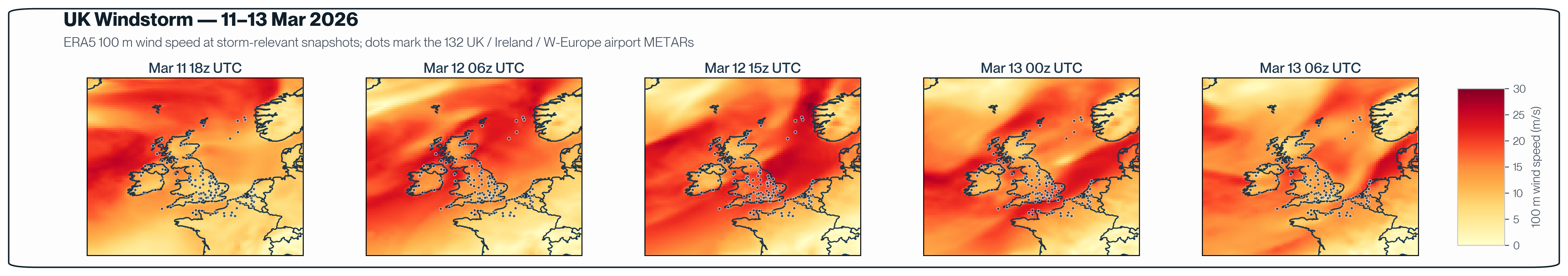
The heat map above traces the storm's evolution: the system intensifying through March 11, peaking across the UK and adjacent North Sea around midday on March 12, and gradually clearing through March 13. It was a broad Atlantic system tracking eastward across the UK, the kind of multi-day wind ramp where forecast skill across several days, not just the hours immediately ahead, shapes positioning and scheduling decisions across power and gas markets.
The dots overlaid on each panel are the 250 evaluation points used in this case study: random sample locations distributed across the UK and surrounding seas, with a deliberate mix of onshore and offshore positions to represent the kinds of sites a wind-energy operator might care about. The same 250 locations appear in every snapshot; what changes is the wind field around them.
We ran two parallel evaluations: MetaMesh-Static for 10 m wind speed and MetaMesh-Dynamic for 100 m wind speed. For the sake of simplicity, we refer to both variants as MetaMesh in the rest of the study. See MetaMesh’s blog for more information on its architecture [MetaMesh Blog].
Forecast horizons run from 12 hours out to 360 hours (15 days).
Results
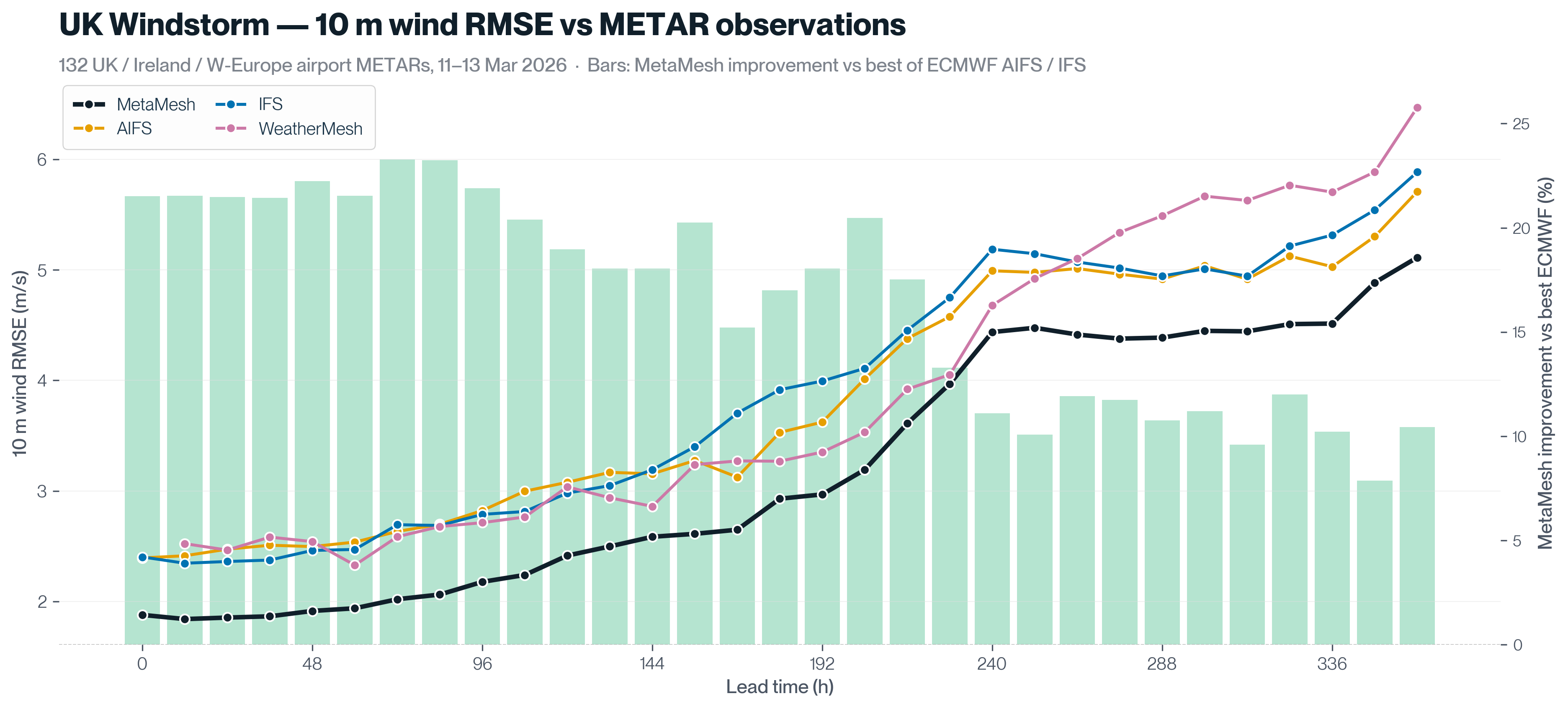
10m wind: Through Day 3, MetaMesh delivered the lowest RMSE, performing ~22% below the better of IFS-Ens and AIFS-Ens at each horizon. The lead held into the medium range (atleast 15% through Day 4-7) and narrowed but did not disappear in the long range (at least 10% through Day 8-15).
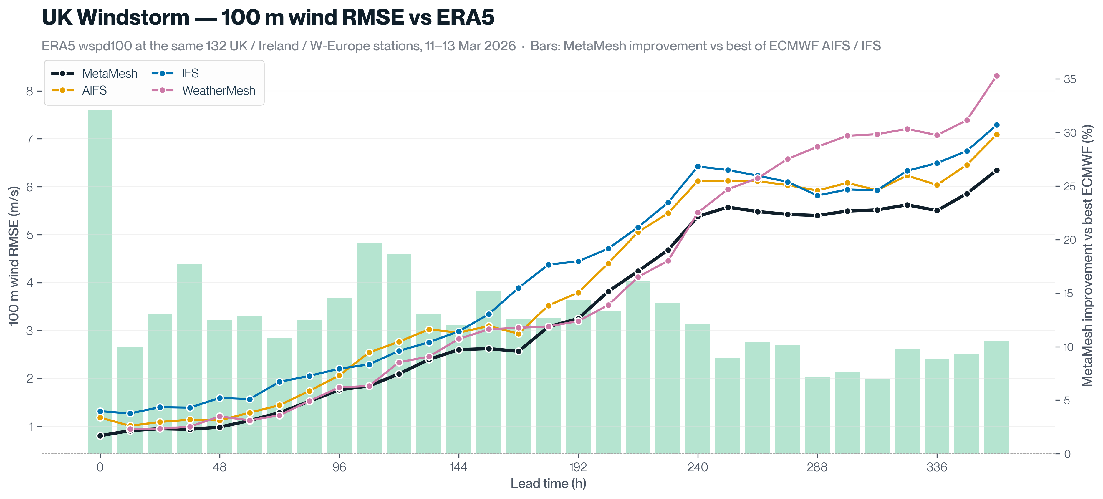
100m wind: The 100m picture mirrors the 10m one; no forecast horizon at which AIFS or IFS overtakes MetaMesh. The long range (Day 8-15) is the weakest performing range for all models, but MetaMesh still holds at least a 7% lead.
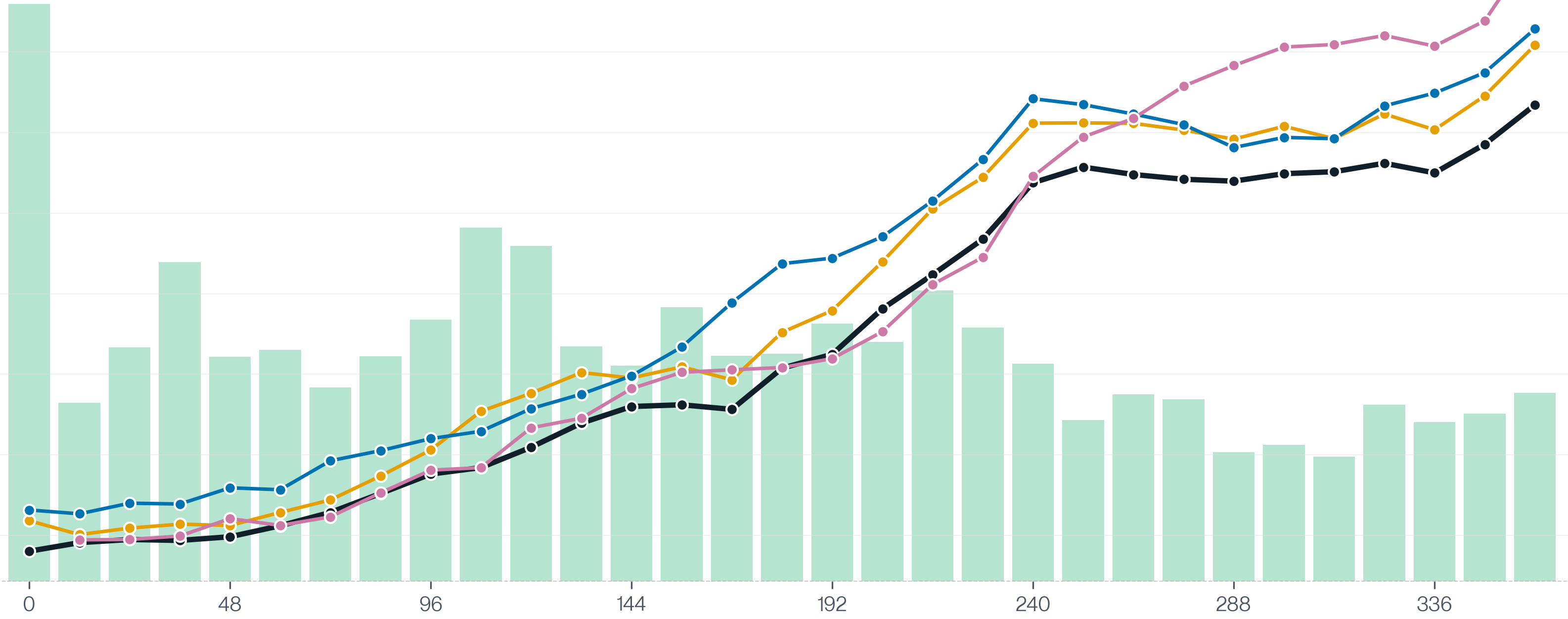
To understand these results, we can look at how the blend is weighting its inputs.
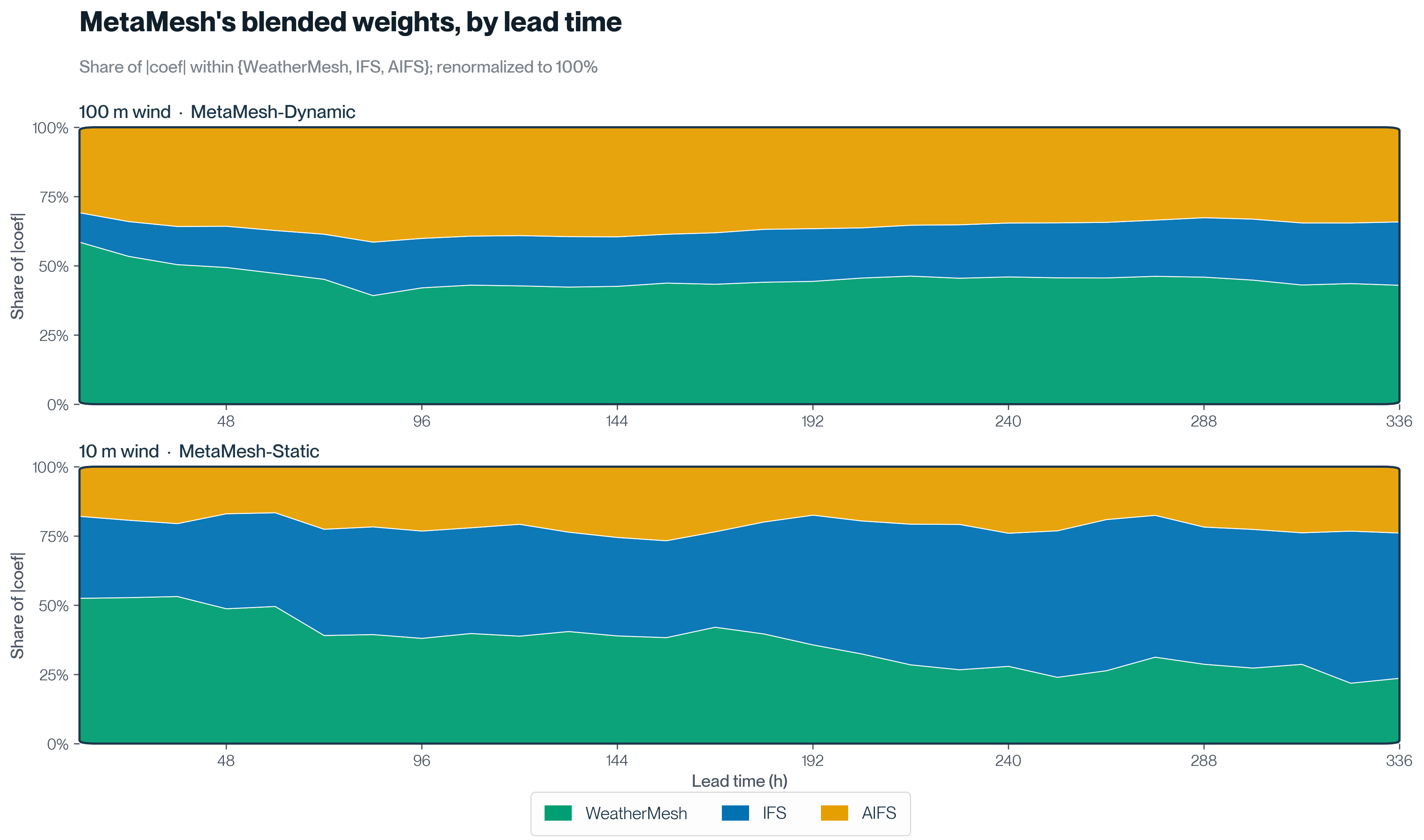
Two patterns explain the result:
- WeatherMesh anchors the blend where MetaMesh is the strongest. In 10m wind for example, MetaMesh’s lead over IFS/AIFS is largest in the first three days of forecast horizon (21-23%). Across the same window, WeatherMesh contributes 49% of the blended weight on average. WeatherMesh anchors the blend where MetaMesh is the strongest. When we look at this 10m wind example, MetaMesh’s lead over IFS/AIFS is largest in the first three days of the forecast horizon (by ~20%). Across the same window, WeatherMesh contributes to almost ~50% of the blended weight on average. Check out WeatherMesh benchmarks here5.
- MetaMesh's dynamic weighting, made possible by its architecture. In 100m wind for example, WeatherMesh stays the largest single contributor at every lead, but the relative balance shifts across the forecast horizon: MetaMesh's blend rebalances toward IFS and AIFS. Where most blends apply fixed weights on a fixed schedule ("60% IFS, 40% GFS"), MetaMesh learns weights that vary by lead time, variable, and region, recalibrates them daily, and re-blends as new input models publish.
Final thoughts
No single forecast model is best at everything (yet). Each has its strengths, its blind spots, and a window of lead times where it leads. The case for a multi-model blend is to recognize that honestly and combine inputs in a way no single model can replicate.
The March 11-13 retrospective is one example. Across the entire 1 to 15 day window, MetaMesh outperformed both ECMWF models at the 10m and 100m windspeed RMSE. WeatherMesh anchored the blend at short range and IFS and AIFS picked up more weight as lead time grew. Because MetaMesh's weights are recalibrated daily, the same retrospective re-run a few months from now would apply different weights and likely show different margins. That's by design: the blend is built to track which models are performing best in the recent past rather than freezing a snapshot.
Case studies like this motivates our team to keep advancing the blending architecture, expanding the input set, and growing the global balloon network that feeds WeatherMesh underneath it all.
To see how MetaMesh would have called a specific event in your own portfolio, get in touch with our team.


